Author: Jeff Blackadar

This is a note about how I connected to box.com using its API so that a python program could download images and meta data.

Details of the API are here https://developer.box.com/en/guides/authentication/oauth2/with-sdk/

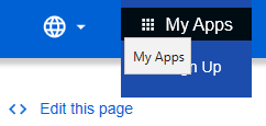
To connect to Box, I needed to make an app. See the link “My Apps” in the SDK link above.

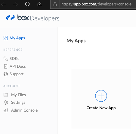
Create a new app.

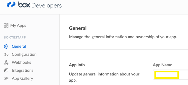
Give your app a name.

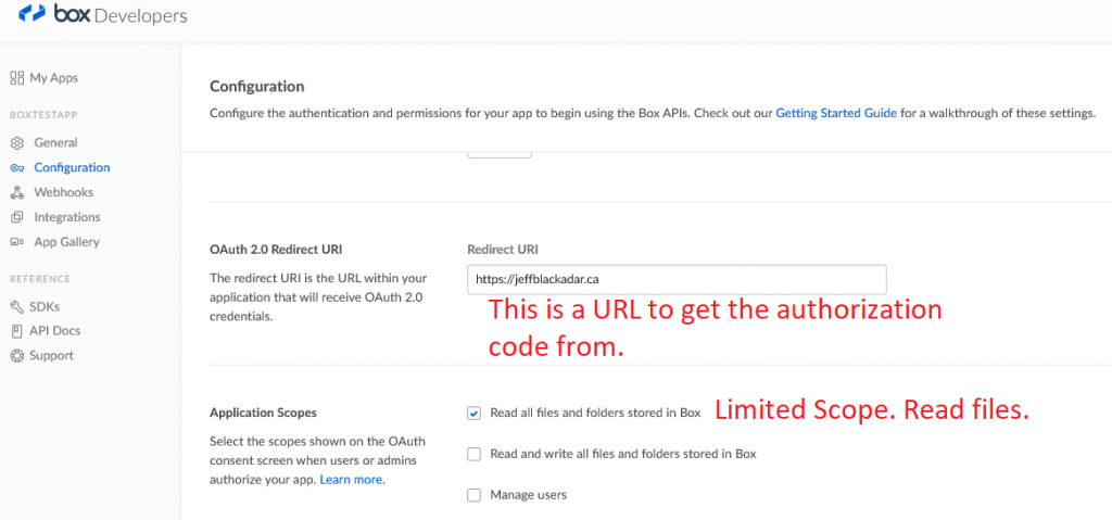
I used OAuth 2.0 Authentication

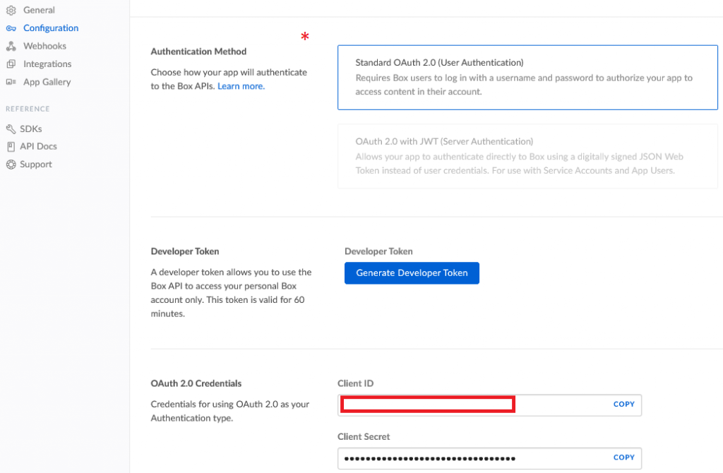
I put the client_id and client_secret values into a json file that looks like this:

{
"client_id":"ryyyyyyyyyyyyyyyyyyyyyyyyyyyyyyy",
"client_secret":"Vzzzzzzzzzzzzzzzzzzzzzzzzzzzzzzz"
}

Here is the code to connect:

!pip install boxsdk
!pip install auth
!pip install redis
!pip install mysql.connector
!pip install requests

from boxsdk import OAuth2

import json
#Set the file we want to use for authenticating a Box app
#The json file stores the client_id and client_secret so we don't have it in the code.
# The json file looks like this:
#{
#"client_id":"___the_codes_for_client_id___",
#"client_secret":"___the_codes_for_client_secret___"
#}

oauth_settings_file = 'C:\\ProgramData\\box_app_test.json'
with open(oauth_settings_file, "r") as read_file:
    oauth_data = json.load(read_file)
print(oauth_data["client_id"])
print(oauth_data["client_secret"])

oauth = OAuth2(
    client_id=oauth_data["client_id"],
    client_secret=oauth_data["client_secret"]
)

auth_url, csrf_token = oauth.get_authorization_url('https://jeffblackadar.ca')
print("Click on this:")
print(auth_url)
print(csrf_token)
print("Copy the code that follows code= in the URL.  Paste it into the oauth.authenticate('___the_code___') below.  Be quick, the code lasts only a few seconds.")

I ran the code above in a Jupyter notebook. The output is:

ryyyyyyyyyyyyyyyyyyyyyyyyyyyyyyy
 Vzzzzzzzzzzzzzzzzzzzzzzzzzzzzzzz
 Click on this:
 https://account.box.com/api/oauth2/authorize?state=box_csrf_token_Qcccccccccccccccccccccc&response_type=code&client_id=ryyyyyyyyyyyyyyyyyyyyyyyyyyyyyyy&redirect_uri=https%3A%2F%2Fjeffblackadar.ca
 box_csrf_token_Qcccccccccccccccccccccc
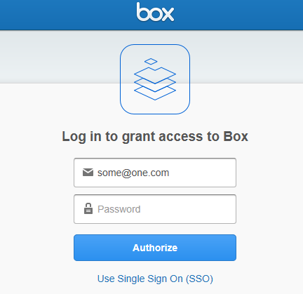
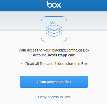
 Copy the code that follows code= in the URL.  Paste it into the oauth.authenticate('the_code') below.  Be quick, the code lasts only a few seconds.

You will notice the Redirect URI set above appears when the URL above is clicked. But first you must authenticate with Box.com using your password to make sure only authorized users read your content.

Paste the code above into the statement below. You need to work quickly, the code is valid for a few seconds only. There is a better way to do this, but this is what is working at this time, please let me know of improvements.

from boxsdk import Client

# Make sure that the csrf token you get from the `state` parameter
# in the final redirect URI is the same token you get from the
# get_authorization_url method to protect against CSRF vulnerabilities.
#assert 'THE_CSRF_TOKEN_YOU_GOT' == csrf_token
access_token, refresh_token = oauth.authenticate('qzzzzzzzzzzzzzzzzzzzzzzzzzzzzzzzzzz')
client = Client(oauth)

Then run this test. It will list all of the files in the folders on box.com.

def process_subfolder_test(client, folder_id, folder_name):
    print("this folder: "+folder_name)
    items = client.folder(folder_id=folder_id).get_items()
    for item in items:
        print('{0} {1} is named "{2}"'.format(item.type.capitalize(), item.id, item.name))
        if(item.type.capitalize()=="Folder"):
            process_subfolder_test(client, item.id,folder_name+"/"+item.name)
        if(item.type.capitalize()=="File"):
            #print(item)
            print('File: {0} is named: "{1}" path: {2} '.format(item.id, item.name, folder_name+"/"+item.name))            
    return

process_subfolder_test(client, '0',"")

Here is the test output:

this folder: 
Folder 98208868103 is named "lop"
this folder: /lop
Folder 98436941432 is named "1963"
this folder: /lop/1963
File 588118649408 is named "Elizabeth II young 2019-08-10 15_41_20.591925.jpg"
File: 588118649408 is named: "Elizabeth II young 2019-08-10 15_41_20.591925.jpg" path: /lop/1963/Elizabeth II young 2019-08-10 15_41_20.591925.jpg 
File 588114839194 is named "Elizabeth II young 2019-08-10 15_41_52.188758.jpg"
File: 588114839194 is named: "Elizabeth II young 2019-08-10 15_41_52.188758.jpg" path: /lop/1963/Elizabeth II young 2019-08-10 15_41_52.188758.jpg 
File 587019307270 is named "eII2900.png"
File: 587019307270 is named: "eII2900.png" path: /lop/eII2900.png 
File 587019495720 is named "eII2901.png"
File: 587019495720 is named: "eII2901.png" path: /lop/eII2901.png 
File 587019193229 is named "eII2903.png"
File: 587019193229 is named: "eII2903.png" path: /lop/eII2903.png 

I processed 1458 models in this spreadsheet (see models tab). As mentioned in my previous post, these are the parameters:

• model_number – the identification number
• batch_size – the size of the batch. 8 or 16
• filters1 – the number of filters for layer 1. (possible values 32,64 or 128)

model.add(Conv2D(filters=filters1, 

• dropout1 – Dropout (if greater than 0) (possible values 0,0.25,0.5)

if(dropout1>0):
model.add(Dropout(dropout1))

• filters2 – the number of filters for layer 2. (32,64 or 128)
• dropout2 – dropout for layer 2. (0,0.25,0.5)
• filters3 – the number of filters for layer 3. (32,64 or 128)
• dropout3 – dropout for layer 3. (0,0.25,0.5)
• loss – the result of running the model.
• accuracy – (as above.)

A review of the spreadsheet shows that many of the models I ran have poor accuracy, even as low as 1:3 (0.333333333333333) to predict a match between three coin obverse portraits (Elizabeth II, George VI and Abraham Lincoln). I did find some models with an accuracy above 80% yet I wanted to see if there were patterns I could use to improve my set of models. So I used a Seaborn heatmap of the models (below) for batch sizes of 8,16 and both together.

The heatmap for loss and accuracy to the model parameters in the last two rows shows there is a slightly negative relationship between accuracy and dropout1. It is possible it would be more efficient to use dropout values of 0 or 0.25 and not 0.5 when running these models again. It also seems like there is a slightly positive relationship between batch size and accuracy possibly indicating that larger batch sizes may lead to more accurate models. I have been running a set of models with a batch size of 32 to see if this pattern becomes stronger. (same spreadsheet, models tab.) I am also going to validate my approach through additional personal (not machine) learning.

In Deep Learning for Python, François Chollet provides a “universal workflow of machine learning”. (Chapter 4, page 114.) I have been using his steps to seek the best performing image recognition model. I tried iterations of various models with different numbers of layers, filters and dropouts. An example of a model that did not provide a satisfactory level of accuracy is below.

def createModel5fail2():

    #tried kernel_size=(5,5), 

    from keras import models
    model = models.Sequential()    

    model.add(Conv2D(filters=32, 
               kernel_size=(5,5), 
               strides=(1,1),
               padding='same',
               input_shape=(image_width, image_height,NB_CHANNELS),
               data_format='channels_last'))
    model.add(Activation('relu'))
    model.add(MaxPooling2D(pool_size=(2,2),
                     strides=2))

    model.add(Conv2D(filters=64,
               kernel_size=(5,5),
               strides=(1,1),
               padding='valid'))
    model.add(Activation('relu'))
    model.add(MaxPooling2D(pool_size=(2,2),
                     strides=2))
    
    model.add(Flatten())        
    model.add(Dense(128))
    model.add(Activation('relu'))

    model.add(Dropout(0.25))
    
    #number of classes
    # 1,0,0 E-II
    # 0,1,0 G-VI
    # 0,0,1 G-VI
    model.add(Dense(3, activation='softmax'))

    return model 

In order to be more methodical and record my results I added a spreadsheet of model parameters (see models tab). These are the parameters:

• model_number – the identification number
• batch_size – the size of the batch. 8 or 16
• filters1 – the number of filters for layer 1.

model.add(Conv2D(filters=filters1, 

• dropout1 – Dropout (if greater than 0)

if(dropout1>0):
model.add(Dropout(dropout1))

• filters2 – the number of filters for layer 2.
• dropout2 – dropout for layer 2.
• filters3 – the number of filters for layer 3.
• dropout3 – dropout for layer 3.
• loss – the result of running the model.
• accuracy – (as above.)

The code to create the spreadsheet of parameters is here. (It’s just nested loops.) Below is the code to create a model from parameters fed from the spreadsheet. In the course of writing up this post, I found 2 bugs in the code below that are now corrected. Because of the bugs I need to re-run my results.

def createModelFromSpreadsheet():

    from keras import models
    model = models.Sequential()
    

    model.add(Conv2D(filters=filters1, 
               kernel_size=(2,2), 
               strides=(1,1),
               padding='same',
               input_shape=(image_width, image_height,NB_CHANNELS),
               data_format='channels_last'))
    model.add(Activation('relu'))
    model.add(MaxPooling2D(pool_size=(2,2),
                     strides=2))
    if(dropout1>0):
        model.add(Dropout(dropout1))
    
    model.add(Conv2D(filters=filters2,
               kernel_size=(2,2),
               strides=(1,1),
               padding='valid'))
    model.add(Activation('relu'))
    model.add(MaxPooling2D(pool_size=(2,2),
                     strides=2))

    if(dropout2>0):
        model.add(Dropout(dropout2))

    if(filters3>0): 
        model.add(Conv2D(filters=filters3,
               kernel_size=(2,2),
               strides=(1,1),
               padding='valid'))
        model.add(Activation('relu'))
        model.add(MaxPooling2D(pool_size=(2,2),
                     strides=2))

        if(dropout3>0):
            model.add(Dropout(dropout3))

    
    model.add(Flatten())        
    model.add(Dense(512))
    model.add(Activation('relu'))
    model.add(Dropout(0.25))
    
    #number of classes
    # 1,0,0 E-II
    # 0,1,0 G-VI
    # 0,0,1 G-VI
    model.add(Dense(3, activation='softmax'))

    return model
  

Below is the code to loop through each row of the model spreadsheet, create a model from the parameters, fit it and record the result.

number_of_models_to_run = 40
for number_of_models_to_run_count in range (0,number_of_models_to_run):
    model_row = int(worksheet_config.cell(1, 2).value)

    BATCH_SIZE = int(worksheet_models.cell(model_row, 2).value,0) #, 'batch_size')
    filters1 = int(worksheet_models.cell(model_row, 3).value,0) #, 'filters1')
    dropout1 = float(worksheet_models.cell(model_row, 4).value) #, 'dropout1')
    filters2 = int(worksheet_models.cell(model_row, 5).value,0) #, 'filters2')
    dropout2 = float(worksheet_models.cell(model_row, 6).value) #, 'dropout2')
    filters3 = int(worksheet_models.cell(model_row, 7).value,0) #, 'filters3')
    dropout3 = float(worksheet_models.cell(model_row, 8).value) #, 'dropout3')

    print(str(model_row)+" "+str(BATCH_SIZE)+" "+str(filters1)+" "+str(dropout1)+" "+str(filters2)+" "+str(dropout2)+" "+str(filters3)+" "+str(dropout3))
    # NB_CHANNELS = # 3 for RGB images or 1 for grayscale images
    NB_CHANNELS =  1
    NB_TRAIN_IMG = 111
    # NB_VALID_IMG = # Replace with the total number validation images  
    NB_VALID_IMG = 54


    #*************
    #* Change model
    #*************
    model2 = createModelFromSpreadsheet()
    model2.compile(optimizer='rmsprop', loss='categorical_crossentropy', metrics=['accuracy'])
    model2.summary()

    epochs = 100

    # Fit the model on the batches generated by datagen.flow().
    history2 = model2.fit_generator(datagen.flow(tr_img_data , tr_lbl_data, batch_size=BATCH_SIZE),
                                  #steps_per_epoch=int(np.ceil(tr_img_data .shape[0] / float(batch_size))),
                                  steps_per_epoch=NB_TRAIN_IMG//BATCH_SIZE,
                                  epochs=epochs,
                                  validation_data=(val_img_data, val_lbl_data),
                                  validation_steps=NB_VALID_IMG//BATCH_SIZE,
                                  shuffle=True,
                                  workers=4)

    evaluation = model2.evaluate(tst_img_data, tst_lbl_data)
    print(evaluation)
    print(evaluation[0])
    #record results
    worksheet_models.update_cell(model_row, 10, evaluation[0])
    worksheet_models.update_cell(model_row, 11, evaluation[1])
    worksheet_config.update_cell(1, 2, str(model_row+1))
    if(evaluation[1]>0.75):
        number_of_models_to_run_count = number_of_models_to_run
        print("Good Model - stopped")

In the course of running these models, I had a model that provided 77% image recognition accuracy when tested and so I saved the weights. Due to the bugs I found I am re-running my results now to see if I can reproduce the model and find a better one.

Since the start of September I have been working to improve my image classification model. The positive result is that I have a model that is capable of categorizing 3 different types of coins, however the model is not yet as accurate as it needs to be. For reference here is my working code

Categorizing three different types of coin images.

I have added photos of Abraham Lincoln to the collection of coin photos I am using for training. Each class of photo is “one hot label” encoded to give it an identifier that can be used in the model: 1,0,0 = Elizabeth; 0,1,0 = George VI and 0,0,1 = Abraham Lincoln. (Continuing this pattern, additional classes of coins can be added for training.) Below is the code that does this based on the first three characters of the photo’s file name.

def one_hot_label(img):
     label = img.split('.')[0]
     label = label[:3]
     if label == 'eII':
         ohl = np.array([1,0,0])
     elif label == 'gvi':
         ohl = np.array([0,1,0])
     elif label == 'lin':
         ohl = np.array([0,0,1])
     return ohl

The model I have trained can recognize Abraham Lincoln more times that it does not.

Model Accuracy

When training the model I monitor the loss and accuracy for both training and validation. Validation accuracy is where the model checks its effectiveness against a set of validation images. Training accuracy is a measure of how well the model is performing using its training data. A model is functioning well if its training accuracy and validation accuracy are both high .

 Epoch 16/150 13/13 [==============================] - 0s 23ms/step - loss: 0.8050 - acc: 0.5769 - val_loss: 10.7454 - val_acc: 0.3333 

As shown above, at this point in the training of this model, the training accuracy (acc:) is low (57.6%) and the validation accuracy (val_acc:) is even lower (33%). For an image prediction between 3 different types of coins, this model is validated to be as accurate as rolling a die.

The red line of the training accuracy in the graph above shows a model that becomes more accurate over time. The accuracy of the model is very low initially, but it does climb almost continuously.

The validation accuracy of the model also begins quite low. Consider the area of the graph inside the magenta box denoted by (T). During this training, val_acc stalls at 33% between epochs 5 and 25. During my experiments with different model configurations, if I saw this stall happen I would terminate the training to save time. Considering what happened here, I should let the models run longer. This model eventually achieved a validation accuracy of 78%, the best result I had in the past couple of days.

Overfitting

The validation accuracy of this model peaks at epoch 88. As it declines, the training accuracy of the model continues a trend to higher accuracy. This is a sign that the model is overfitting and training for features that are present in the training data but won’t be generally present for other images. An overfit model is not useful for recognizing images from outside of its training set. This information is useful since it signifies that this model should be trained for approximately 88 epochs and not 150. At the same time, this particular model still needs work. Even with a validation accuracy of 77%, the model is still likely overfit given it has a training accuracy of 90%. So it is likely that this model will make errors of prediction when used with new images of our coin subjects.

An objective of this research is to demonstrate a means to automatically classify an image of an artifact using computer vision. I am using a method and code from Dattaraj Rao’s book Keras to Kubernetes: The Journey of a Machine Learning Model to Production. In Chapter 5 he demonstrates the use of machine learning to classify logo images of Pepsi and Coca Cola. I have used his code in an attempt to classify coin images of George VI and Elizabeth II.

Code for this is here: https://github.com/jeffblackadar/image_work/blob/master/Keras_to_Kubernetes_Rao.ipynb

The images I am using are here.

Below are my initial results; the prediction is shown below the image.

…So far so good…

As noted above, this prediction failed.

I am not sure why yet, but here is my experience so far. On my first run through, the prediction failed for the first image of George VI too. I got the correct result when I used a larger image size for training and validation.

train_generator = train_datagen.flow_from_directory(
        training_dir,
        target_size=(300, 300),

(above) The original code uses an image size of 150 x 150 so I doubled it in each line of the program where that size is used. I may need to use a larger size than 300 x 300.

The colours of my coin images are somewhat uniform, while Rao’s example uses Coke’s red and white logo versus Pepsi’s logo with blue in it. Does color play a more significant role in image classification using Keras than I thought? I will look at what is happening during model training to see if I can address this issue.

Data Augmentation

I have a small number of coin images yet effective training of an image recognition model requires numerous different images. Rao uses the technique of data augmentation to manipulate a small set of images into a larger set of images that can be used for training by distorting them. This can be particularly useful when training a model to recognize images taken by cameras from different angles as would happen in outdoor photography. A portion of Rao’s code is below. Given the coin images I am using are photographed from above, I have reduced the level of distortion (shear, zoom, width and height shift.)

#From:
# Keras to Kubernetes: The Journey of a Machine Learning Model to Production
# Dattaraj Jagdish Rao
# Pages 152-153

 from keras.preprocessing.image import ImageDataGenerator
 import matplotlib.pyplot as plt
 %matplotlib inline
 training_dir = "/content/drive/My Drive/coin-image-processor/portraits/train"
 validation_dir = "/content/drive/My Drive/coin-image-processor/portraits/validation"
 gen_batch_size = 1
 This is meant to train the model for images taken at different angles.  I am going to assume pictures of coins are from directly above, so there is little variation
 train_datagen = ImageDataGenerator(
     rescale=1./255,
     shear_range=0.05,
     zoom_range=0.05,
     fill_mode = "nearest",    
     width_shift_range=0.05,
     height_shift_range=0.05,
     rotation_range=20,
     horizontal_flip=False)
 train_generator = train_datagen.flow_from_directory(
         training_dir,
         target_size=(300, 300),
         batch_size=32,
         class_mode='binary')
 class_names = ['elizabeth_young','george_vi']
 print ("generating images")
 ROW = 10
 plt.figure(figsize=(20,20))
 for i in range(ROW*ROW):
     plt.subplot(ROW,ROW,i+1)
     plt.xticks([])
     next_set = train_generator.next()
     plt.imshow(next_set[0][0])
     plt.xticks([])
     plt.yticks([])
     plt.grid(False)
     plt.xlabel(class_names[int(next_set[1][0])])
 plt.show()

My next steps to improve the results I am getting are looking at what is happening as the models are trained and training the models longer using larger image sizes.

References

Rao, Dattaraj. Keras to Kubernetes: The Journey of a Machine Learning Model to Production. 2019.

[1 – footnote] This test image is from a Google search. The original image is from: https://www.cdncoin.com/1937-1964-60-Coin-Set-in-Case-p/20160428003.htm

I have a few dozen pictures of Elizabeth II from Canadian 1 cent pieces. I want to see if I can train a model that can in-paint a partial image. Haiyan Wang, Zhongshi He, Dingding Chen, Yongwen Huang, and Yiman He have written an excellent study of this technique in their article “Virtual Inpainting for Dazu Rock Carvings Based on a Sample Dataset” in the Journal on Computing and Cultural Heritage. [1]

I am using Mathias Gruber’s PConv-Keras repository https://github.com/MathiasGruber/PConv-Keras in GitHub to do image inpainting. He has impressive results and as a caveat for my results, I am not yet training the model used for inpainting nearly as long as Gruber does. I am using Google Colab and it is not meant for long running processes so I am using a small number of steps and epochs to train the model. Even with this constraint I am seeing potential results.

The steps used to setup Mathias Gruber’s PConv-Keras in Google Colab are here. Thanks to Eduardo Rosas for these instructions so I could get this set up.

Using Gruber’s PConv-Keras I have been able to train a model to perform image inpainting. My next steps are to refine the model, train it more deeply and look for improved results. The code and results I am working on are on my Google Drive at this time. The images I am using are here.

This week I improved the program to process coin images as well. I see improved results by having a higher tolerance of impurities in the background of the picture when finding whitespace. (I use white_mean = 250, not 254 or 255) This version is in GitHub.

1 Wang, Haiyan, Zhongshi He, Dingding Chen, Yongwen Huang, and Yiman He. 2019. “Virtual Inpainting for Dazu Rock Carvings Based on a Sample Dataset.” Journal on Computing and Cultural Heritage 12 (3): 1-17.

As mentioned in previous posts, I need numerous images to train an image recognition model. My goal is to have many examples of the image of Elizabeth II like the one below. To be efficient, I want to process many photographs of 1 cent coins using a program and so that program must be able to reliably find the centre of the portrait.

To crop the image I used two methods: 1. remove whitespace from the outside inward and 2. find the edge of the coin using OpenCV’s cv2.HoughCircles Function.

Removing whitespace from the outside inward is the simpler of the two methods. To do this I assume the edges of the image are white, color 255 in a grayscale image. If the mean value of pixel colors is 255 for a whole column of pixels, that whole column can be considered whitespace. If the mean value of pixel colors is lower than 255 I assume the column contains part of the darker coin. Cropping the image from the x value of this column will crop the whitespace from the left edge of the image.

for img_col_left in range(1,round(gray_img.shape[1]/2)):
    if np.mean(gray_img,axis = 0)[img_col_left] < 254:
        break 

The for loop of this code starts from the first pixel and moves toward the center. If the mean of the column is less than 254 the loop stops since the edge of the coin is found. I am using 254 instead of 255 to allow for some specks of dust or other imperfections in the white background. Using a for loop is not efficient and this code should be improved, but I want to get this working first.

Before the background is cropped, the image is converted to black and white and then grayscale in order to simplify the edges. Here is the procedure at this point.

import numpy as np
import cv2
import time
from google.colab.patches import cv2_imshow

def img_remove_whitespace(imgo):
    print("start " + str(time.time()))
    #convert to black and white - make it simpler?
    # define a threshold, 128 is the middle of black and white in grey scale
    thresh = 128

    # assign blue channel to zeros
    img_binary = cv2.threshold(imgo, thresh, 255, cv2.THRESH_BINARY)[1]
    #cv2_imshow(img_binary) 
    
    gray_img = cv2.cvtColor(img_binary, cv2.COLOR_BGR2GRAY)
    #cv2_imshow(gray_img) 
    print(gray_img.shape)

    # Thanks https://likegeeks.com/python-image-processing/
    # croppedImage = img[startRow:endRow, startCol:endCol]
      
    # allow for 254 (slightly less than every pixel totally white to allow some specks)
    #count in from the right edge until the mean of each column is less than 255
    for img_row_top in range(0,round(gray_img.shape[0]/2)):    
        if np.mean(gray_img,axis = 1)[img_row_top] < 254:
            break 
    print(img_row_top)
    for img_row_bottom in range(gray_img.shape[0]-1,round(gray_img.shape[0]/2),-1):
        if np.mean(gray_img,axis = 1)[img_row_bottom] < 254:
          break 
    print(img_row_bottom)    
    for img_col_left in range(1,round(gray_img.shape[1]/2)):
        if np.mean(gray_img,axis = 0)[img_col_left] < 254:
            break 
    print(img_col_left)    
    for img_col_right in range(gray_img.shape[1]-1,round(gray_img.shape[1]/2),-1):
        if np.mean(gray_img,axis = 0)[img_col_right] < 254:
            break
    print(img_col_right)
          
    imgo_cropped = imgo[img_row_top:img_row_bottom,img_col_left:img_col_right,0:3]
    print("Whitespace removal")
    print(imgo_cropped.shape)
    
    # cv2_imshow(imgo_cropped) 
    print("end " + str(time.time()))
    return(imgo_cropped)

A problem with this method is that some images have shadows which interfere with the procedure from seeing the true edge of the coin. (See below.)

For cases like the image above, I tried to use OpenCV’s Hough Circles to find the boundary of the coin. Thanks to Adrian Rosebrock’s tutorial “Detecting Circles in Images using OpenCV and Hough Circles” I was able to apply this here.

In my case, cv2.HoughCircles found too many circles. For example, it found 95 of them in one image. Almost all of these circles are not the edge of the coin. I used several methods to try to find the circle that represented the edge of the coin. I sorted the circles by radius, reasoning the largest circle was the edge. It was not always. I looked for large circles that were completely inside the image but also got erroneous results. (See below.) Perhaps I am using this incorrectly, but I have decided this method is not reliable enough to be worthwhile so I am going to stop using it. The code to use the Hough circles is below. Warning, there is likely a problem with it.

print("Since finding whitespace did not work, we will find circles. This will take more time")      
circles = cv2.HoughCircles(gray_img, cv2.HOUGH_GRADIENT, 1.2, 100)

# ensure at least some circles were found
if circles is not None:
    print("Circles")
    print(circles.shape)

    # convert the (x, y) coordinates and radius of the circles to integers
    circles = np.round(circles[0, :]).astype("int")
    circles2=sorted(circles,key=takeThird,reverse=True)
    print("There are " + str(len(circles2)) +" circles found in this image")
    for cir in range(0,len(circles2)):    
        x = circles2[cir][0]
        y = circles2[cir][1]
        r = circles2[cir][2]
        print()
        if r < good_coin_radius*1.1 and r > good_coin_radius*0.9:
            if (x > (good_coin_radius*0.9) and x < (output.shape[0]-(good_coin_radius*0.9))):
                if (y > (good_coin_radius*0.9) and y < (output.shape[1]-(good_coin_radius*0.9))):
                    print("I believe this is the right circle.")  
                    print(circles2[cir])
                    cv2.circle(output, (x, y), r, (0, 255, 0), 4)        
                    cv2.rectangle(output, (x - 5, y - 5), (x + 5, y + 5), (0, 128, 255), -1)  
                    cv2_imshow(output)
                    output = output[x-r:x+r,y-r:y+r]
                    width_half = round(output.shape[0]/2)
                    height_half = round(output.shape[1]/2)
                    cv2.circle(output,(width_half, height_half), round(r*1.414).astype("int"), (255,255,255), round(r*1.4).astype("int"))
                    output = img_remove_whitespace(output)
                    cv2_imshow(output)
                    return(output)

My conclusion is that I am only going to use coins from the left half of each picture I take since the photo flash works better there and there are fewer shadows. I will take care to remove debris around the coins that interferes with finding whitespace. Failing that, the routine removes photos that it can’t crop to the expected size of the coin. This results in a loss of some photos, but this is acceptable here since I need don’t need every photo to train the image recognition model. Below is a rejected image. The cleaned up code I am using right now is here.

I would like to train an image recognition model with my own images to see how well it works. Here I want to use the obverse of coins to make a model to recognize the portraits of Elizabeth II (younger), Elizabeth II (more mature), George VI and Abraham Lincoln.

Initially I used 5 cent coins but I found they reflected too much light to take a good photograph so I switched to 1 cent coins. I also started with a camera on a Microsoft Surface Pro computer, taking pictures of 9 coins at a time in order to try to be efficient, but I did not get the higher image quality I believe I need.

The next step is to remove the background using OpenCV in Python, crop the image to have just the coin. I don’t want to have the image recognition model recognize the portrait because her name is printed on it, so I will crop it again to have only the portrait.

I believe this type of image processing can be applied to historical artifacts photographed using a neutral background. I am concerned the coins are too worn and have too little variation in colour to make a good model but that in itself will be useful to learn if it’s the case.

My thanks to the Saskatoon Coin Club for their excellent page describing the obverse designs of Canadian one cent coins.

I am doing research for the Computational Creativity and Archaeological Data project. My current challenge has been to use techniques from Computer Vision to analyse images relevant to Computational Research on the Ancient Near East (CRANE) with the goal to provide additional understanding of these images. Computer Vision and machine learning could identify and classify elements in images or provide a possible reconstruction of a partial artifact using an image of it combined with a model of images of related artifacts. Here, I would like to reference Ivan Tyukin, Konstantin Sofeikov, Jeremy Levesley, Alexander N. Gorban, Penelope Allison and Nicholas J. Cooper’s work “Exploring Automated Pottery Identification [Arch-I-Scan]” in Internet Archaeology 50. https://doi.org/10.11141/ia.50.11

In order to classify images I plan to use machine learning. To do this I need a workable method, a machine learning platform and then to create a model that can be used for image recognition.

The method I plan to use is described in the books Deep Learning with Python/R. Using the techniques from the book, I can train a model to recognize different types of images and so far I have been able to make the examples in the book work.

Google Colab is the machine learning platform I am using. I am comfortable using this given I am not using any sensitive data as per guidelines here. Colab offers a free GPU which is a requirement for the efficient processing of these models. (Training one model was going to take 2 hours without a GPU. With a GPU it took a few seconds.)

Python vs. R. Colab has some support for R but it did not work well enough to install what was required. I have switched to Python. This is the notebook of my setup of Colab.

I have made examples from Deep Learning with Python work. Now I want to create my own sets of training data, train models with them and see the results. This will provide a better understanding of the limitations and pitfalls of using machine learning for image recognition.

I am a fan of fractals and recently I wanted to learn more about object-oriented programming in R using classes. Adam Spannbauer has an excellent tutorial using R6 classes and ggplot2 to create fractal trees and I adapted it for L-system line fractals found in Przemyslaw Prusinkiewicz and Aristid Lindenmayer’s book The Algorithmic Beauty of Plants.

An example of an L-system line fractal follows.

Imagine you are a turtle drawing a line according to instructions: + means turn to the right by 90 degrees. – means turn left 90 degrees. F means move forward a set distance. (Let’s assume it’s 100 pixels.)

So F-F-F-F would draw a square.

F also has a special role in that it replicates itself as a “generator”. If the generator for F is F-F+F+FF-F-F+F then the F-F-F-F would become F-F+F+FF-F-F+F-F-F+F+FF-F-F+F-F-F+F+FF-F-F+F-F-F+F+FF-F-F+F and be drawn like the shape below. Recursion is used to generate subsequent generations of the same repeating pattern which can be seen here.

Images of more fractals are on these pages. This project also allowed me to try Github pages and Binder. The repository for the code used is here: https://github.com/jeffblackadar/fractal.