Month: March 2021

This is a note about replicating the work of Drs. Arnau Garcia‐Molsosa, Hector A. Orengo, Dan Lawrence, Graham Philip, Kristen Hopper and Cameron A. Petrie in their article Potential of deep learning segmentation for the extraction of archaeological features from historical map series. [1]

The authors demonstrate a working process to recognize map text. Their “Detector 3” targets the “word ‘Tell’ in Latin characters.” [1] As they note, “‘tell’ (Arabic for settlement mound) may appear as the name of a mound feature or a toponym in the absence of an obvious topographic feature. This convention may be due to the placement of the names on the map, or a real difference in the location of the named village and the tell site, or because the tell has been destroyed in advance of the mapping of the region.” [1]

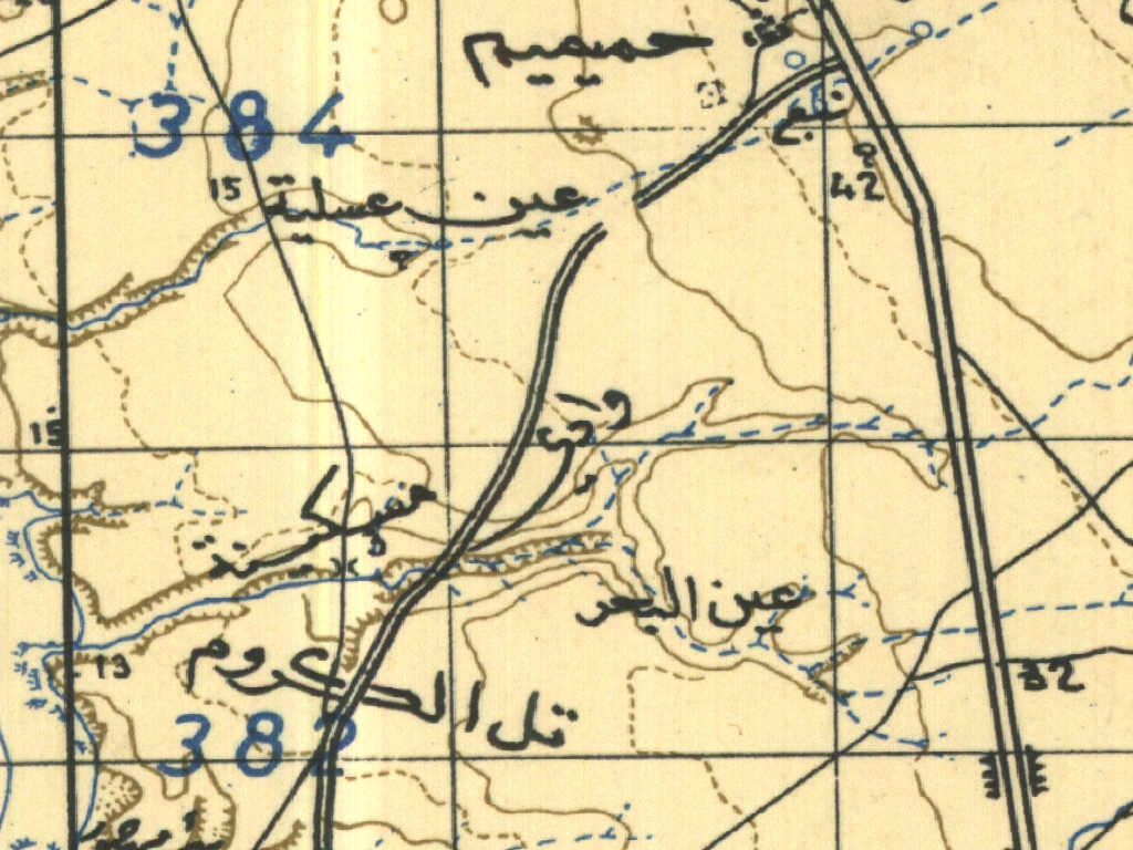
I worked with a georeferenced map provided by Dr Kristen Hopper, Dr. Dan Lawrence and Dr. Hector Orengo: 1:200,000 Levant. Sheet NI-37-VII., Damas. 1941. The map uses Latin characters and so I used Azure Cognitive Services to transcribe the text. Below is part of the map showing “R.R.”, signifying Roman Ruins, and “Digue Romaine”, Roman dike.

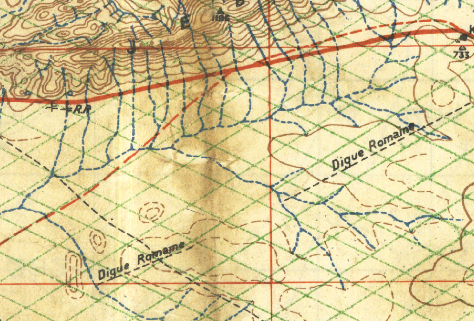
This map contains a lot of text:

After transcription I applied a crude filter to remove numbers and retain places that contained lowercase text romam, roman, romai, digue, ell, r.r. Below is a sample of what was retained:

keep i :  44 Tell Hizime
keep i :  56 Nell Sbate te
keep i :  169 Well Jourdich
keep i :  182 Tell abou ech Chine
keep i :  190 ell Hajan
keep i :  221 Tell Kharno ube
keep i :  240 Deir Mar Ellaso &
keep i :  263 Dique Romam
keep i :  303 Tell Arran
keep i :  308 Digue Romame
keep i :  313 & Tell Bararhite
keep i :  314 788 ou Tell Abed
keep i :  350 R.R.
keep i :  379 Telklaafar in Tell Dothen
keep i :  388 Tell Afair
keep i :  408 Tell el Assouad
keep i :  428 ETell el Antoute
keep i :  430 AiTell Dekova
keep i :  433 Tell' Chehbé
keep i :  436 R.R.
keep i :  437 ptromain bouche, Dein ej Jenoubi
keep i :  438 R.R.
keep i :  439 Tell el Moralla!?

... etc.

Below is a screenshot of georeferenced place names displayed on a satellite image in QGIS:

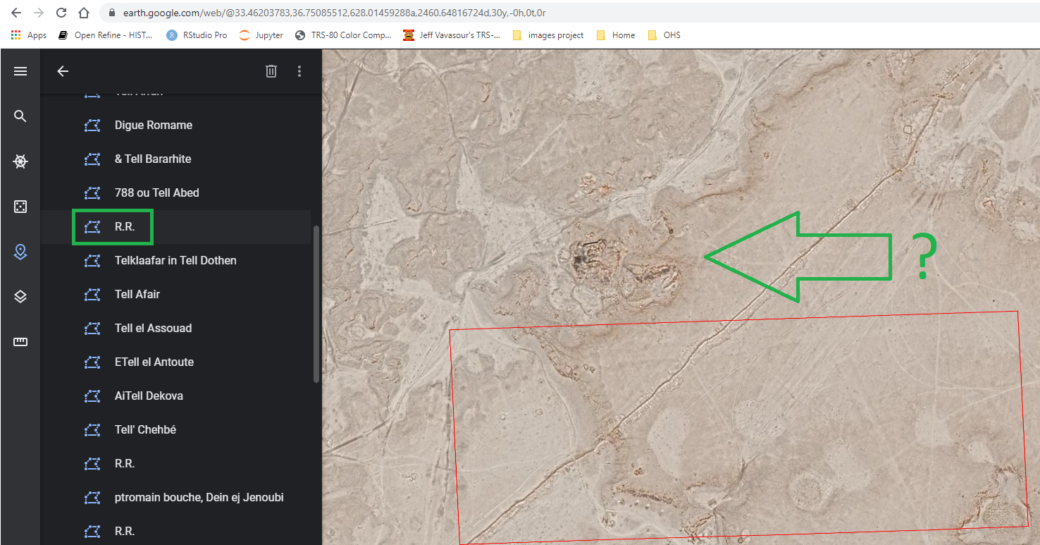
The polygons containing place names are in a shapefile and kml. These locations on the map that possibly represent tells and Roman ruins. The kml can be downloaded and added to Google Earth as a Project, as shown below. This allows an examination of the landscape near each label as seen from a satellite. I have not examined these sites and I don’t have the expertise or evidence to determine whether these are archeological sites. This is meant as a proof of technology to find areas of interest. If you’d like a copy of the kml or shapefile, feel free to contact me on Twitter @jeffblackadar.

The code I used is here.

Thank you to Drs. Kristen Hopper, Dan Lawrence and Hector Orengo for providing these georeferenced maps.

[1] Garcia-Molsosa A, Orengo HA, Lawrence D, Philip G, Hopper K, Petrie CA. Potential of deep learning segmentation for the extraction of archaeological features from historical map series. Archaeological Prospection. 2021;1–13. https://doi.org/10.1002/arp.1807

As noted in an earlier post, I am working with a large set of digital maps thanks to Dr. Kristen Hopper, Dr. Dan Lawrence and Dr. Hector Orengo. As I work through these maps I want to record their attributes so I don’t need to re-open them frequently. This is a note about a process to record metadata in QGIS I am trying out.

For each map I wish to record:

• map_name.
• crs – The geographic coordinate reference system.
• extent – The coordinates of the map’s coverage.
• language – Maps are Arabic, French and English.
• year.
• color_scheme – Most maps have black text, brown topographic features and blue water features. Some maps use red and a few add green.
• ruins_symbol – Some maps use R. R. to signify a Roman Ruin. Others use a picture symbol.

For map_name I use the layer name. Crs and extent are stored as part of the geographic information in the map’s georeferenced tif.

Language can be defined in Layer Properties | Metadata.

I used Metadata Keywords to define color_scheme, ruins_symbol and year.

A small program in QGIS can export the data into a .csv.

This is the export program in QGIS:

from xml.etree import ElementTree as ETree

file_out = open("E:\\a_new_orgs\\crane\\large\\maps_syria.csv", "w")
file_out.write('"map_name","crs","extent","language","year","color_scheme","ruins_symbol"\n')

layers = qgis.utils.iface.mapCanvas().layers()
for layer in layers:
    layerType = layer.type()
    layerName = layer.name()
    if layerType == QgsMapLayer.RasterLayer:
          
        xml = QgsLayerDefinition.exportLayerDefinitionLayers([layer], QgsReadWriteContext()).toString()
        xml_root =  ETree.fromstring(xml)
        
        keywords = {'color_scheme': '', 'year': '', 'ruins_symbol': ''}
        for obj in xml_root.findall('./maplayers/maplayer/resourceMetadata'):
            print(obj)
            map_language = obj.find('language').text
            for keywords_obj in obj.findall('./keywords'):
                keywords[keywords_obj.attrib['vocabulary']] = keywords_obj.find('keyword').text
        print(keywords)
        print(str(layer.name()), layer.crs(), layer.extent())
        file_out.write('"' + str(layer.name()) + '","' + str(layer.crs()) + '","' + str(layer.extent()) + '","' + str(map_language) + '","' +str(keywords['year']) + '","' + keywords['color_scheme']  + '","' + keywords['ruins_symbol'] + '"\n' )

file_out.close()

This map below conveys a lot of information using color. Topographic lines are brown, water features are blue. It’s a visually complex map. I wanted to see if I removed non-text blue and brown features on the map, could I improve optical character recognition of the text in black. This is a quick note about the process.

I used this short program to filter the color so that features in black were retained while lighter colors were changed to white (255,255,255).

import cv2
import numpy as np
# This is the 1 map tile we'll use for this example:
from google.colab.patches import cv2_imshow
img = cv2.imread('/content/drive/MyDrive/crane_maps_syria/maps_large/Djeble_georef/jpg_tiles/r07c09.jpg',-1)
print("before")
cv2_imshow(img)

# Thanks to https://stackoverflow.com/questions/50210304/i-want-to-change-the-colors-in-image-with-python-from-specific-color-range-to-an
hsv=cv2.cvtColor(img,cv2.COLOR_BGR2HSV)

# Define lower and uppper limits of what we call "black"
color_lo=np.array([0,0,0])
color_hi=np.array([90,90,115])

# Mask image to only select black text
mask=cv2.inRange(hsv,color_lo,color_hi)

img[mask==0]=(255,255,255)

cv2.imwrite("result.png",img)
img2 = cv2.imread('result.png',-1)

print("after")
cv2_imshow(img2)

Below is the result of transcription and there is no visible benefit here. However this appears to be a useful method for separating analysis of map elements using color.